
Hints to deal with Missing Values in R
In R missing values are usually, but not always, represented by letters NA. How to deal with missing values is very important in the data analytics world. Missing data can be sometimes tricky while analyzing a data frame, since it should be handled correctly for our statistical analysis. Before diving into more complex details about missing data, the first question that should be asked in any exploratory data analysis is: Do I have missing values in my database?
First, we need to load the libraries needed for our analysis.
library(Amelia)
library(tidyr)
library(readxl)
library(tidyimpute)
library(mice)
library(VIM)
library(dplyr)
library(here)
Next, we will load the data frame related to the NFL Positional Salaries from 2011 to 2018.
nfl <- read_excel(here::here("nfl_salaries.xlsx"))
glimpse(nfl)
## Observations: 800
## Variables: 11
## $ year <dbl> 2011, 2011, 2011, 2011, 2011, 2011, 2011, ...
## $ Cornerback <dbl> 11265916, 11000000, 10000000, 10000000, 10...
## $ `Defensive Lineman` <dbl> 17818000, 16200000, 12476000, 11904706, 11...
## $ Linebacker <dbl> 16420000, 15623000, 11825000, 10083333, 10...
## $ `Offensive Lineman` <dbl> 15960000, 12800000, 11767500, 10358200, 10...
## $ Quarterback <dbl> 17228125, 16000000, 14400000, 14100000, 13...
## $ `Running Back` <dbl> 12955000, 10873833, 9479000, 7700000, 7500...
## $ Safety <dbl> 8871428, 8787500, 8282500, 8000000, 780433...
## $ `Special Teamer` <dbl> 4300000, 3725000, 3556176, 3500000, 325000...
## $ `Tight End` <dbl> 8734375, 8591000, 8290000, 7723333, 697466...
## $ `Wide Receiver` <dbl> 16250000, 14175000, 11424000, 11415000, 10...Now that the data is loaded, let’s use some nice functions from Base R to answer the question mentioned above. The first function we could use is is.na(). This function tells us for each observation if the existence of missing values is TRUE or FALSE. However, when we have a multitude of cases it is not very clear if our question was answered. Instead, we should use any(is.na(name of dataframe)) or sum(is.na(name of the dataframe)).
any(is.na(nfl))## [1] TRUEsum(is.na(nfl))## [1] 56any(is.na(nfl)) says TRUE, meaning we have missing data. Besides, sum(is.na(nfl)) tells us that we have in total 56 missing values.
Even though our question was answered, we still do not know where the missing values are present. More specifically, in which variables do we have missing values? That’s our second question.
For that, there are some functions available. We can use the which(is.na()) function.
which(is.na(nfl))## [1] 4098 4099 4100 4189 4190 4191 4192 4193 4194 4195 4196 4197 4198 4199
## [15] 4200 4294 4295 4296 4297 4298 4299 4300 4390 4391 4392 4393 4394 4395
## [29] 4396 4397 4398 4399 4400 4498 4499 4500 4596 4597 4598 4599 4600 4698
## [43] 4699 4700 4790 4791 4792 4793 4794 4795 4796 4797 4798 4799 4800 6500However, this gives only the location in terms of number of case and nothing about the variable where the missing data is present. We can use for this the colSums() function.
colSums(is.na(nfl))## year Cornerback Defensive Lineman Linebacker
## 0 0 0 0
## Offensive Lineman Quarterback Running Back Safety
## 0 55 0 0
## Special Teamer Tight End Wide Receiver
## 1 0 0We can now see that we have 55 missing values in the Quarterback position and 1 missing value in the Special Teamer position. Nonetheless, we can visually check where in our variables we have missing data. The missmap() function from the Amelia package is fit for this purpose.
missmap(nfl)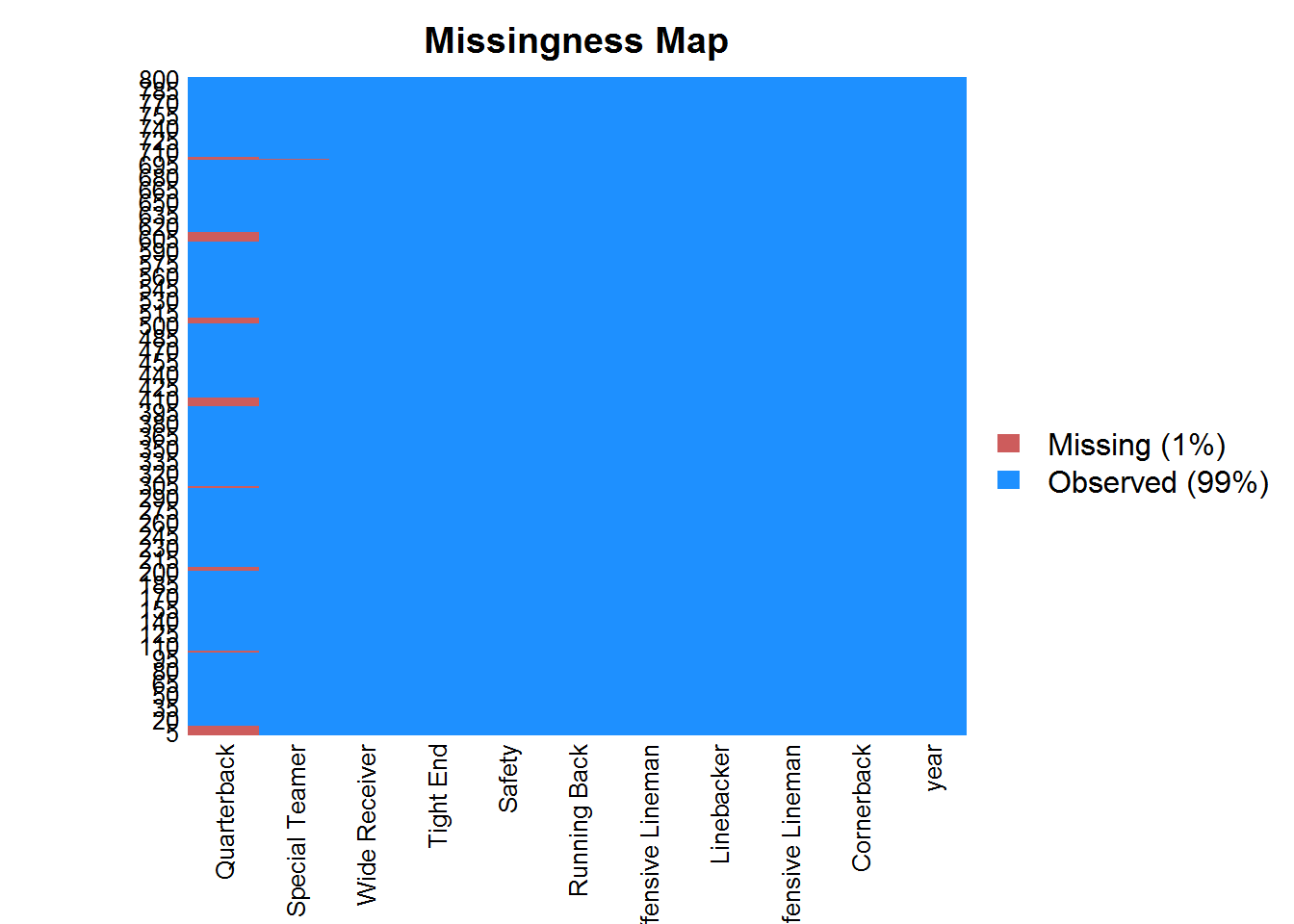
Visually we can check that we have only missing values in the Quarterback and Special Teamer columns. Another alternative is to check where exactly are the missing values and their correspondent proportion in total. Now, we should use aggr() function from the VIM package.
plot <- aggr(nfl, col = c("green", "red"),
             numbers = TRUE,
             sortVars = TRUE)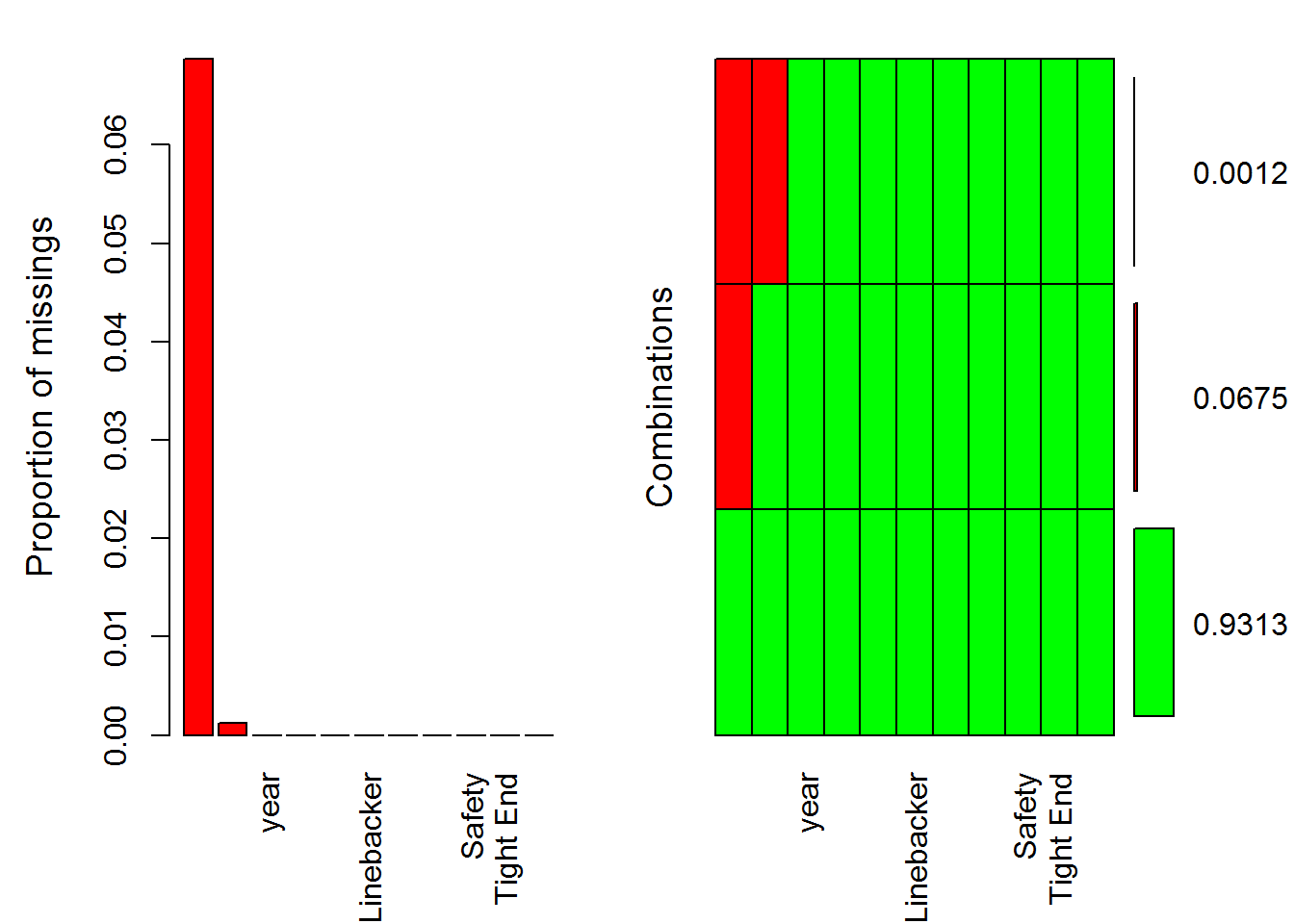
##
##  Variables sorted by number of missings:
##           Variable   Count
##        Quarterback 0.06875
##     Special Teamer 0.00125
##               year 0.00000
##         Cornerback 0.00000
##  Defensive Lineman 0.00000
##         Linebacker 0.00000
##  Offensive Lineman 0.00000
##       Running Back 0.00000
##             Safety 0.00000
##          Tight End 0.00000
##      Wide Receiver 0.00000
The values in the table show that 6.875% of the cases in the Quarterback variable correspond to missing values, while only 0.125% correspond to missing values in the Special Teamer variable. The plot does not show all the variable names because of some issue that I could not solve. Nonetheless, from the table it is clear the proportion of missing values in each variable.
Now the last step anwers the third question: What should I do with the missing values? The simplest and more direct way to deal with missing data is to omit it from our data frame. In this case, we can use the na.omit() function.
nfl_complete <- na.omit(nfl)
any(is.na(nfl_complete))
## [1] FALSEThe downside being the deletion of too many observations of our data which could have been useful to our analysis. In this case, we could delete only missing values of a specific variable. To do that, go ahead and use the drop_na() function form the tidyr() package.
nfl %>%
  drop_na("Special Teamer")
## # A tibble: 799 x 11
## year Cornerback `Defensive Line~ Linebacker `Offensive Line~
## <dbl> <dbl> <dbl> <dbl> <dbl>
## 1 2011 11265916 17818000 16420000 15960000
## 2 2011 11000000 16200000 15623000 12800000
## 3 2011 10000000 12476000 11825000 11767500
## 4 2011 10000000 11904706 10083333 10358200
## 5 2011 10000000 11762782 10020000 10000000
## 6 2011 9244117 11340000 8150000 9859166
## 7 2011 8000000 10000000 7812500 9500000
## 8 2011 7900000 9482500 7700000 9420000
## 9 2011 7400000 8450000 7200000 8880000
## 10 2011 7000000 8383266 7100000 8686750
## # ... with 789 more rows, and 6 more variables: Quarterback <dbl>,
## # `Running Back` <dbl>, Safety <dbl>, `Special Teamer` <dbl>, `Tight
## # End` <dbl>, `Wide Receiver` <dbl>In the example, we have deleted all missing values corresponding to the Special Teamer column.
Two other neat functions from the tidyr() package can also be of great help. The fill() and replace_na() can impute values where before were missing values. The fill() function allows to replace the missing values with the most recent non-missing value present before or after the missing value. There is an argument in this function called .direction which enables you to choose if it is the nearest value being displayed before or after the missing value.
If we write the code as follows:
nfl %>%
  fill(Quarterback, .direction = "down")
## # A tibble: 800 x 11
## year Cornerback `Defensive Line~ Linebacker `Offensive Line~
## <dbl> <dbl> <dbl> <dbl> <dbl>
## 1 2011 11265916 17818000 16420000 15960000
## 2 2011 11000000 16200000 15623000 12800000
## 3 2011 10000000 12476000 11825000 11767500
## 4 2011 10000000 11904706 10083333 10358200
## 5 2011 10000000 11762782 10020000 10000000
## 6 2011 9244117 11340000 8150000 9859166
## 7 2011 8000000 10000000 7812500 9500000
## 8 2011 7900000 9482500 7700000 9420000
## 9 2011 7400000 8450000 7200000 8880000
## 10 2011 7000000 8383266 7100000 8686750
## # ... with 790 more rows, and 6 more variables: Quarterback <dbl>,
## # `Running Back` <dbl>, Safety <dbl>, `Special Teamer` <dbl>, `Tight
## # End` <dbl>, `Wide Receiver` <dbl>With .direction = “down”, it will show (?) the value appearing before the missing value which will fill the NA values, but if we write with .direction = “up” the reserve will occur. Meaning, the value being displayed after the NA value will fill the space where the missing value once was.
nfl %>%
  fill(Quarterback, .direction = "up")
## # A tibble: 800 x 11
## year Cornerback `Defensive Line~ Linebacker `Offensive Line~
## <dbl> <dbl> <dbl> <dbl> <dbl>
## 1 2011 11265916 17818000 16420000 15960000
## 2 2011 11000000 16200000 15623000 12800000
## 3 2011 10000000 12476000 11825000 11767500
## 4 2011 10000000 11904706 10083333 10358200
## 5 2011 10000000 11762782 10020000 10000000
## 6 2011 9244117 11340000 8150000 9859166
## 7 2011 8000000 10000000 7812500 9500000
## 8 2011 7900000 9482500 7700000 9420000
## 9 2011 7400000 8450000 7200000 8880000
## 10 2011 7000000 8383266 7100000 8686750
## # ... with 790 more rows, and 6 more variables: Quarterback <dbl>,
## # `Running Back` <dbl>, Safety <dbl>, `Special Teamer` <dbl>, `Tight
## # End` <dbl>, `Wide Receiver` <dbl>Rather, if we want to replace the missing value with the mean or median of the respective variable we could use replace_na.
# with the mean
nfl %>%
  replace_na(replace = list(Quarterback = mean(.$Quarterback, na.rm =TRUE),
             `Special Teamer` = mean(.$`Special Teamer`, na.rm =TRUE)))
## # A tibble: 800 x 11
## year Cornerback `Defensive Line~ Linebacker `Offensive Line~
## <dbl> <dbl> <dbl> <dbl> <dbl>
## 1 2011 11265916 17818000 16420000 15960000
## 2 2011 11000000 16200000 15623000 12800000
## 3 2011 10000000 12476000 11825000 11767500
## 4 2011 10000000 11904706 10083333 10358200
## 5 2011 10000000 11762782 10020000 10000000
## 6 2011 9244117 11340000 8150000 9859166
## 7 2011 8000000 10000000 7812500 9500000
## 8 2011 7900000 9482500 7700000 9420000
## 9 2011 7400000 8450000 7200000 8880000
## 10 2011 7000000 8383266 7100000 8686750
## # ... with 790 more rows, and 6 more variables: Quarterback <dbl>,
## # `Running Back` <dbl>, Safety <dbl>, `Special Teamer` <dbl>, `Tight
## # End` <dbl>, `Wide Receiver` <dbl># with the median
nfl %>%
replace_na(replace = list(Quarterback = median(.$Quarterback, na.rm =TRUE),
`Special Teamer` = median(.$`Special Teamer`, na.rm =TRUE)))## # A tibble: 800 x 11
## year Cornerback `Defensive Line~ Linebacker `Offensive Line~
## <dbl> <dbl> <dbl> <dbl> <dbl>
## 1 2011 11265916 17818000 16420000 15960000
## 2 2011 11000000 16200000 15623000 12800000
## 3 2011 10000000 12476000 11825000 11767500
## 4 2011 10000000 11904706 10083333 10358200
## 5 2011 10000000 11762782 10020000 10000000
## 6 2011 9244117 11340000 8150000 9859166
## 7 2011 8000000 10000000 7812500 9500000
## 8 2011 7900000 9482500 7700000 9420000
## 9 2011 7400000 8450000 7200000 8880000
## 10 2011 7000000 8383266 7100000 8686750
## # ... with 790 more rows, and 6 more variables: Quarterback <dbl>,
## # `Running Back` <dbl>, Safety <dbl>, `Special Teamer` <dbl>, `Tight
## # End` <dbl>, `Wide Receiver` <dbl>A more elegant approach - I believe - to substitute missing values with the mean or median is to use the functions available in the package tidyimpute. As the code below shows, it`s very simple to impute the mean or median to our missing values.
# with mean
nfl %>%
  impute_mean(Quarterback, `Special Teamer`)
## # A tibble: 800 x 11
## year Cornerback `Defensive Line~ Linebacker `Offensive Line~
## <dbl> <dbl> <dbl> <dbl> <dbl>
## 1 2011 11265916 17818000 16420000 15960000
## 2 2011 11000000 16200000 15623000 12800000
## 3 2011 10000000 12476000 11825000 11767500
## 4 2011 10000000 11904706 10083333 10358200
## 5 2011 10000000 11762782 10020000 10000000
## 6 2011 9244117 11340000 8150000 9859166
## 7 2011 8000000 10000000 7812500 9500000
## 8 2011 7900000 9482500 7700000 9420000
## 9 2011 7400000 8450000 7200000 8880000
## 10 2011 7000000 8383266 7100000 8686750
## # ... with 790 more rows, and 6 more variables: Quarterback <dbl>,
## # `Running Back` <dbl>, Safety <dbl>, `Special Teamer` <dbl>, `Tight
## # End` <dbl>, `Wide Receiver` <dbl># with the median
nfl %>%
impute_median(Quarterback, `Special Teamer`)## # A tibble: 800 x 11
## year Cornerback `Defensive Line~ Linebacker `Offensive Line~
## <dbl> <dbl> <dbl> <dbl> <dbl>
## 1 2011 11265916 17818000 16420000 15960000
## 2 2011 11000000 16200000 15623000 12800000
## 3 2011 10000000 12476000 11825000 11767500
## 4 2011 10000000 11904706 10083333 10358200
## 5 2011 10000000 11762782 10020000 10000000
## 6 2011 9244117 11340000 8150000 9859166
## 7 2011 8000000 10000000 7812500 9500000
## 8 2011 7900000 9482500 7700000 9420000
## 9 2011 7400000 8450000 7200000 8880000
## 10 2011 7000000 8383266 7100000 8686750
## # ... with 790 more rows, and 6 more variables: Quarterback <dbl>,
## # `Running Back` <dbl>, Safety <dbl>, `Special Teamer` <dbl>, `Tight
## # End` <dbl>, `Wide Receiver` <dbl>And that’s it for today’s post! I hope this mini tutorial helps you in dealing with missing values in R. Thanks for reading us and keep coding in R.
