
Combine Data frames in R
Sometimes, before we start to explore our data, we need to put them together. For instance, we might have them stored in different data frames and we have to join variables from two or more data frames in one. This post will talk about the different functions we can use to achieve that goal. We will be using the dplyr package to combine different data frames.
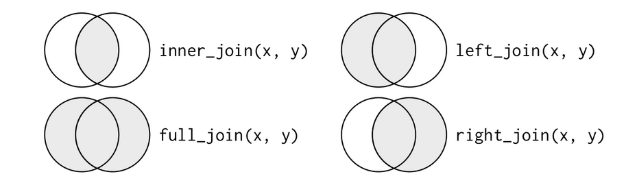
Firstly, we will show examples related to what is called mutating joins. These joins combine two data frames by matching observations in common variables.
Mutating Joins
For this tutorial I have created small datasets just for the sole purpose of writing this blog. Therefore, the data was created by myself and if there is any relationship between the variables, it is not real.
Here you can see a Venn diagram of the different types of mutating joins (source: http://r4ds.had.co.nz/relational-data.html):
First, we will load the packages and data frames needed for this tutorial.
library(here)
library(tibble)
library(tidyverse) # load packages related to data cleaning(in this tutorial dplyr for joins and set operators,  and purrr to use the reduce() function)
library(readxl) # load excel files
# dataframes
df1 <- read_excel(here::here("df1.xlsx"))
df2 <- read_excel(here::here("df2.xlsx"))
df3 <- read_excel(here::here("df3.xlsx"))
df4 <- read_excel(here::here("df4.xlsx"))
Let us start with the data frames df1 and df2.
df1:
df1 ## # A tibble: 9 x 5
## Id Face Sex Dom Str
## <dbl> <chr> <chr> <dbl> <dbl>
## 1 1 A Female 3 3
## 2 2 B Female 5 4
## 3 3 C Female 6 5
## 4 4 D Female 7 6
## 5 5 E Female 8 1
## 6 6 F Female 1 3
## 7 7 G Male 3 4
## 8 8 H Male 4 2
## 9 9 I Male 5 3df2:
df2## # A tibble: 9 x 5
## Id Face Sex Nationality SES
## <dbl> <chr> <chr> <chr> <chr>
## 1 1 L Female PT Low
## 2 2 B Female DEU Middle
## 3 3 M Female PT High
## 4 4 D Female PT Millionaire
## 5 5 E Female PT Low
## 6 6 F Female UK Low
## 7 7 G Male UK High
## 8 8 H Male USA Middle
## 9 9 I Male USA MiddleIf our goal is to maintain all elements of df1 and the elements of df2 in common with df1, we should use a left_join(). We can see that we have 3 variables in common. Our code for this is the following:
df_left <- df1 %>%
  left_join(df2, by = c("Id", "Face", "Sex"))# use of by argument where we write the common variables in both datasets

df_left
## # A tibble: 9 x 7
## Id Face Sex Dom Str Nationality SES
## <dbl> <chr> <chr> <dbl> <dbl> <chr> <chr>
## 1 1 A Female 3 3 <NA> <NA>
## 2 2 B Female 5 4 DEU Middle
## 3 3 C Female 6 5 <NA> <NA>
## 4 4 D Female 7 6 PT Millionaire
## 5 5 E Female 8 1 PT Low
## 6 6 F Female 1 3 UK Low
## 7 7 G Male 3 4 UK High
## 8 8 H Male 4 2 USA Middle
## 9 9 I Male 5 3 USA MiddleAs you can see the output maintains all the columns, but we have 2 missing values in the Nationality and SES columns because the first and third elements of df2 on the Face and Sex columns were different from df1. As said before, a left_join() maintains all elemens of df1 and the common elements between df2 and df1.
Sometimes, we might just want to do the reverse, maintain all elements of df2 and elements of df1 in common with df2. For that you should use a right_join() as the one below:
df_right <- df2 %>%
  right_join(df1, by = c("Id", "Face", "Sex"))

df_right
## # A tibble: 9 x 7
## Id Face Sex Nationality SES Dom Str
## <dbl> <chr> <chr> <chr> <chr> <dbl> <dbl>
## 1 1 A Female <NA> <NA> 3 3
## 2 2 B Female DEU Middle 5 4
## 3 3 C Female <NA> <NA> 6 5
## 4 4 D Female PT Millionaire 7 6
## 5 5 E Female PT Low 8 1
## 6 6 F Female UK Low 1 3
## 7 7 G Male UK High 3 4
## 8 8 H Male USA Middle 4 2
## 9 9 I Male USA Middle 5 3In other situations we might want to maintain only the elements in common between df1 and df2. For that you use an inner_join():
df_inner <- df1 %>%
  inner_join(df2, by = c("Id", "Face", "Sex"))

df_inner
## # A tibble: 7 x 7
## Id Face Sex Dom Str Nationality SES
## <dbl> <chr> <chr> <dbl> <dbl> <chr> <chr>
## 1 2 B Female 5 4 DEU Middle
## 2 4 D Female 7 6 PT Millionaire
## 3 5 E Female 8 1 PT Low
## 4 6 F Female 1 3 UK Low
## 5 7 G Male 3 4 UK High
## 6 8 H Male 4 2 USA Middle
## 7 9 I Male 5 3 USA MiddleAs you can see, elements in the first and third columns disappear from our database as they are not common between df1 and df2. In those cases where we want to maintain all observations from df1 and df2, we should go with a full_join():
df_full <- df1 %>%
  full_join(df2, by = c("Id", "Face", "Sex"))

df_full
## # A tibble: 11 x 7
## Id Face Sex Dom Str Nationality SES
## <dbl> <chr> <chr> <dbl> <dbl> <chr> <chr>
## 1 1 A Female 3 3 <NA> <NA>
## 2 2 B Female 5 4 DEU Middle
## 3 3 C Female 6 5 <NA> <NA>
## 4 4 D Female 7 6 PT Millionaire
## 5 5 E Female 8 1 PT Low
## 6 6 F Female 1 3 UK Low
## 7 7 G Male 3 4 UK High
## 8 8 H Male 4 2 USA Middle
## 9 9 I Male 5 3 USA Middle
## 10 1 L Female NA NA PT Low
## 11 3 M Female NA NA PT HighWe have two additional rows. Why? Because with a full join the non-common elements in rows 1 and 3 are added to the joined database.
Very Important NOTES to consider in two situations:
1st situation You may have common variables in two different datasets with different names as in df1 and df4
df1:
df1## # A tibble: 9 x 5
## Id Face Sex Dom Str
## <dbl> <chr> <chr> <dbl> <dbl>
## 1 1 A Female 3 3
## 2 2 B Female 5 4
## 3 3 C Female 6 5
## 4 4 D Female 7 6
## 5 5 E Female 8 1
## 6 6 F Female 1 3
## 7 7 G Male 3 4
## 8 8 H Male 4 2
## 9 9 I Male 5 3And df4:
df4 ## # A tibble: 9 x 5
## Id face_stimuli Sex Nationality SES
## <dbl> <chr> <chr> <chr> <chr>
## 1 1 L Female PT Low
## 2 2 B Female DEU Middle
## 3 3 M Female PT High
## 4 4 D Female PT Millionaire
## 5 5 E Female PT Low
## 6 6 F Female UK Low
## 7 7 G Male UK High
## 8 8 H Male USA Middle
## 9 9 I Male USA MiddleThe variables Face and face_stimuli are the same, but have different names. In that case you should do the following (in this example, we are using an inner_join(), but we could use another type of join):
df_sit1 <- df1 %>%
  inner_join(df4, by = c("Id", "Sex",
                         "Face" = "face_stimuli"))# you make explicit that face equals item

df_sit1
## # A tibble: 7 x 7
## Id Face Sex Dom Str Nationality SES
## <dbl> <chr> <chr> <dbl> <dbl> <chr> <chr>
## 1 2 B Female 5 4 DEU Middle
## 2 4 D Female 7 6 PT Millionaire
## 3 5 E Female 8 1 PT Low
## 4 6 F Female 1 3 UK Low
## 5 7 G Male 3 4 UK High
## 6 8 H Male 4 2 USA Middle
## 7 9 I Male 5 3 USA Middle2nd situation We have variables with the same name, but are not exactly the same. In these two data frames I have created, df5 and df6, we have the counting of white blood cells before and after treatment, respectively.
df5:
df5 <- tibble(Id = 1:10,
             WhiteBloodCell = c(900, 910, 1000, 250, 300, 600, 300, 800, 200, 100),
             SES = c("Middle Class", "Middle Class", "Middle Class", "Upper Middle Class",
                     "Middle Class", "Middle Class", "Middle Class", "Upper Middle Class",
                     "Lower Middle Class", "Lower Middle Class"))

df5
## # A tibble: 10 x 3
## Id WhiteBloodCell SES
## <int> <dbl> <chr>
## 1 1 900 Middle Class
## 2 2 910 Middle Class
## 3 3 1000 Middle Class
## 4 4 250 Upper Middle Class
## 5 5 300 Middle Class
## 6 6 600 Middle Class
## 7 7 300 Middle Class
## 8 8 800 Upper Middle Class
## 9 9 200 Lower Middle Class
## 10 10 100 Lower Middle ClassAnd df6:
df6 <- tibble(Id = 1:10,
             WhiteBloodCell = c(1000, 980, 1200, 500,
                                500, 700, 300, 1000, 400, 300))
df6
## # A tibble: 10 x 2
## Id WhiteBloodCell
## <int> <dbl>
## 1 1 1000
## 2 2 980
## 3 3 1200
## 4 4 500
## 5 5 500
## 6 6 700
## 7 7 300
## 8 8 1000
## 9 9 400
## 10 10 300In these cases, we should follow the function described below:
df_sit2 <- df5 %>%
  left_join(df6, by = c("Id"), suffix = c("Before Treatment", "After Treatment"))#we have in common the variables Id and whitebloodcell, but the latter corresponds to two different elements, before and after treatment.

df_sit2
## # A tibble: 10 x 4
## Id `WhiteBloodCellBefore Tre~ SES `WhiteBloodCellAfter Tre~
## <int> <dbl> <chr> <dbl>
## 1 1 900 Middle Class 1000
## 2 2 910 Middle Class 980
## 3 3 1000 Middle Class 1200
## 4 4 250 Upper Middle~ 500
## 5 5 300 Middle Class 500
## 6 6 600 Middle Class 700
## 7 7 300 Middle Class 300
## 8 8 800 Upper Middle~ 1000
## 9 9 200 Lower Middle~ 400
## 10 10 100 Lower Middle~ 300Filtering Joins
Let’s go now to another type of joins. The FILTERING joins. They have this name because they filter observations in two different datasets. There are two types of filtering joins: semi_join() and anti_join().
The semi_join() maintains all observations in a data frame (x) which are not matched in another data frame (y):
df_semi <- df1 %>%
  semi_join(df2, by = c("Id", "Face", "Sex"))

df_semi
## # A tibble: 7 x 5
## Id Face Sex Dom Str
## <dbl> <chr> <chr> <dbl> <dbl>
## 1 2 B Female 5 4
## 2 4 D Female 7 6
## 3 5 E Female 8 1
## 4 6 F Female 1 3
## 5 7 G Male 3 4
## 6 8 H Male 4 2
## 7 9 I Male 5 3Rows 1 and 3 disappear and the variables Nationality and SES from df2 are no longer showing in this new dataset. Therefore, this join maintains all variables of j1 and the ones in common with df2. In regard to the observations/cases, it maintains only the matching ones.
The anti_join() maintains only the non-common observations between data frame (x) and data frame (y):
df_anti <- df1 %>%
  anti_join(df2, by = c("Id", "Face", "Sex"))

df_anti
## # A tibble: 2 x 5
## Id Face Sex Dom Str
## <dbl> <chr> <chr> <dbl> <dbl>
## 1 1 A Female 3 3
## 2 3 C Female 6 5In this case, only rows 1 and 3 are maintained.
Joining more than 2 data frames
Unfortunately, the mutating and filtering joins only enable the merger of two data frames. However, there are situations where we have 3 or more datasets. Let’s imagine we wanted to join df1, df2, and df3. In this scenario, we would need the reduce() function from the purrr package.
First step is to create a list with the 3 data frames:
a <- list(df1, df2, df3)#create a list with the 3 datasetsAfterwards we write the function below:
df_reduce <- a %>%
  reduce(left_join, by = c("Id", "Face", "Sex"))#use reduce() function. The first argument is the list created. The second argument is the join that you intend to use.

df_reduce
## # A tibble: 9 x 9
## Id Face Sex Dom.x Str.x Nationality SES Dom.y Str.y
## <dbl> <chr> <chr> <dbl> <dbl> <chr> <chr> <dbl> <dbl>
## 1 1 A Female 3 3 <NA> <NA> NA NA
## 2 2 B Female 5 4 DEU Middle NA NA
## 3 3 C Female 6 5 <NA> <NA> NA NA
## 4 4 D Female 7 6 PT Millionaire 7 6
## 5 5 E Female 8 1 PT Low 8 1
## 6 6 F Female 1 3 UK Low 1 3
## 7 7 G Male 3 4 UK High 3 4
## 8 8 H Male 4 2 USA Middle 4 2
## 9 9 I Male 5 3 USA Middle 5 3Set Operations
Sometimes we do not need to use joins when we have two datasets we want to unite. This happens when two datasets have the same variables. For instance, df1 and df3:
See df1:
df1## # A tibble: 9 x 5
## Id Face Sex Dom Str
## <dbl> <chr> <chr> <dbl> <dbl>
## 1 1 A Female 3 3
## 2 2 B Female 5 4
## 3 3 C Female 6 5
## 4 4 D Female 7 6
## 5 5 E Female 8 1
## 6 6 F Female 1 3
## 7 7 G Male 3 4
## 8 8 H Male 4 2
## 9 9 I Male 5 3And df3:
df3## # A tibble: 9 x 5
## Id Face Sex Dom Str
## <dbl> <chr> <chr> <dbl> <dbl>
## 1 10 A Male 8 4
## 2 15 B Male 9 3
## 3 13 C Male 10 8
## 4 4 D Female 7 6
## 5 5 E Female 8 1
## 6 6 F Female 1 3
## 7 7 G Male 3 4
## 8 8 H Male 4 2
## 9 9 I Male 5 3To combine these datasets we should use what is called set operators. R has 3 of such: union, setdiff, and intersect.
union() is used when we want all the unique observations of the two data frames
df_u <- df1 %>%
  union(df3)

df_u
## # A tibble: 12 x 5
## Id Face Sex Dom Str
## <dbl> <chr> <chr> <dbl> <dbl>
## 1 4 D Female 7 6
## 2 2 B Female 5 4
## 3 10 A Male 8 4
## 4 15 B Male 9 3
## 5 1 A Female 3 3
## 6 7 G Male 3 4
## 7 8 H Male 4 2
## 8 13 C Male 10 8
## 9 5 E Female 8 1
## 10 6 F Female 1 3
## 11 3 C Female 6 5
## 12 9 I Male 5 3Now, we have only 12 rows, because 6 of the rows in df3 were the same as in df1. Remember, the union function returns only the unique rows. In this case, we have 12 observations that are unique within both data frames.
In other cases, we can use the setdiff() if we want only the observation in df1 not in common with df3.
df_dif <- df1 %>%
  setdiff(df3)

df_dif
## # A tibble: 3 x 5
## Id Face Sex Dom Str
## <dbl> <chr> <chr> <dbl> <dbl>
## 1 1 A Female 3 3
## 2 2 B Female 5 4
## 3 3 C Female 6 5Returns only the rows with Id 1 to 3. The rows not in common with df3.
Finally, we can use intersect() if we want only the observations in common between df1, df3.
df_intersect <- df1 %>%
  intersect(df3)

df_intersect
## # A tibble: 6 x 5
## Id Face Sex Dom Str
## <dbl> <chr> <chr> <dbl> <dbl>
## 1 4 D Female 7 6
## 2 5 E Female 8 1
## 3 6 F Female 1 3
## 4 7 G Male 3 4
## 5 8 H Male 4 2
## 6 9 I Male 5 3Adding Rows and Columns
Occasionally, it may happen that you want to combine cases from two datasets with the same variables. In that scenario you should use the function bind_rows() from the dplyr package.
We can use the function bind_rows with df1 and df3.
df_bind <- df1 %>%
  bind_rows(df3)

df_bind
## # A tibble: 18 x 5
## Id Face Sex Dom Str
## <dbl> <chr> <chr> <dbl> <dbl>
## 1 1 A Female 3 3
## 2 2 B Female 5 4
## 3 3 C Female 6 5
## 4 4 D Female 7 6
## 5 5 E Female 8 1
## 6 6 F Female 1 3
## 7 7 G Male 3 4
## 8 8 H Male 4 2
## 9 9 I Male 5 3
## 10 10 A Male 8 4
## 11 15 B Male 9 3
## 12 13 C Male 10 8
## 13 4 D Female 7 6
## 14 5 E Female 8 1
## 15 6 F Female 1 3
## 16 7 G Male 3 4
## 17 8 H Male 4 2
## 18 9 I Male 5 3Now we have 18 rows. One nice feature of bind_rows() is the possibility to add an extra column , allowing you to identify of which data frame came each observation.
bind_df2 <- bind_rows(Dataset1 = df1,
                   Dataset2 = df3,
                   .id = "Dataset")

bind_df2
## # A tibble: 18 x 6
## Dataset Id Face Sex Dom Str
## <chr> <dbl> <chr> <chr> <dbl> <dbl>
## 1 Dataset1 1 A Female 3 3
## 2 Dataset1 2 B Female 5 4
## 3 Dataset1 3 C Female 6 5
## 4 Dataset1 4 D Female 7 6
## 5 Dataset1 5 E Female 8 1
## 6 Dataset1 6 F Female 1 3
## 7 Dataset1 7 G Male 3 4
## 8 Dataset1 8 H Male 4 2
## 9 Dataset1 9 I Male 5 3
## 10 Dataset2 10 A Male 8 4
## 11 Dataset2 15 B Male 9 3
## 12 Dataset2 13 C Male 10 8
## 13 Dataset2 4 D Female 7 6
## 14 Dataset2 5 E Female 8 1
## 15 Dataset2 6 F Female 1 3
## 16 Dataset2 7 G Male 3 4
## 17 Dataset2 8 H Male 4 2
## 18 Dataset2 9 I Male 5 3As a result we have a new variable called Dataset with two levels, Dataset1 and Dataset2. This allow us to identify from which dataset the observations came.
Besides rows you can also bind columns. Again, with the package dplyr you have the option of doing it through the bind_cols() function.
Let us use a data frame from another post and break in two:
us_tuition <- read_excel(here("us_avg_tuition.xlsx"))

head(us_tuition)
## # A tibble: 6 x 13
## State `2004-05` `2005-06` `2006-07` `2007-08` `2008-09` `2009-10`
## <chr> <dbl> <dbl> <dbl> <dbl> <dbl> <dbl>
## 1 Alab~ 5683. 5841. 5753. 6008. 6475. 7189.
## 2 Alas~ 4328. 4633. 4919. 5070. 5075. 5455.
## 3 Ariz~ 5138. 5416. 5481. 5682. 6058. 7263.
## 4 Arka~ 5772. 6082. 6232. 6415. 6417. 6627.
## 5 Cali~ 5286. 5528. 5335. 5672. 5898. 7259.
## 6 Colo~ 4704. 5407. 5596. 6227. 6284. 6948.
## # ... with 6 more variables: `2010-11` <dbl>, `2011-12` <dbl>,
## # `2012-13` <dbl>, `2013-14` <dbl>, `2014-15` <dbl>, `2015-16` <dbl># break the data frame in two
us_1 <- us_tuition[1:6]
head(us_1)## # A tibble: 6 x 6
## State `2004-05` `2005-06` `2006-07` `2007-08` `2008-09`
## <chr> <dbl> <dbl> <dbl> <dbl> <dbl>
## 1 Alabama 5683. 5841. 5753. 6008. 6475.
## 2 Alaska 4328. 4633. 4919. 5070. 5075.
## 3 Arizona 5138. 5416. 5481. 5682. 6058.
## 4 Arkansas 5772. 6082. 6232. 6415. 6417.
## 5 California 5286. 5528. 5335. 5672. 5898.
## 6 Colorado 4704. 5407. 5596. 6227. 6284.#
us_2 <- us_tuition[7:13]
head(us_2)## # A tibble: 6 x 7
## `2009-10` `2010-11` `2011-12` `2012-13` `2013-14` `2014-15` `2015-16`
## <dbl> <dbl> <dbl> <dbl> <dbl> <dbl> <dbl>
## 1 7189. 8071. 8452. 9098. 9359. 9496. 9751.
## 2 5455. 5759. 5762. 6026. 6012. 6149. 6571.
## 3 7263. 8840. 9967. 10134. 10296. 10414. 10646.
## 4 6627. 6901. 7029. 7287. 7408. 7606. 7867.
## 5 7259. 8194. 9436. 9361. 9274. 9187. 9270.
## 6 6948. 7748. 8316. 8793. 9293. 9299. 9748.Now let us use the bind_cols() function to unite them.
us_reunited <- us_1 %>%
  bind_cols(us_2)

head(us_reunited)
## # A tibble: 6 x 13
## State `2004-05` `2005-06` `2006-07` `2007-08` `2008-09` `2009-10`
## <chr> <dbl> <dbl> <dbl> <dbl> <dbl> <dbl>
## 1 Alab~ 5683. 5841. 5753. 6008. 6475. 7189.
## 2 Alas~ 4328. 4633. 4919. 5070. 5075. 5455.
## 3 Ariz~ 5138. 5416. 5481. 5682. 6058. 7263.
## 4 Arka~ 5772. 6082. 6232. 6415. 6417. 6627.
## 5 Cali~ 5286. 5528. 5335. 5672. 5898. 7259.
## 6 Colo~ 4704. 5407. 5596. 6227. 6284. 6948.
## # ... with 6 more variables: `2010-11` <dbl>, `2011-12` <dbl>,
## # `2012-13` <dbl>, `2013-14` <dbl>, `2014-15` <dbl>, `2015-16` <dbl>I hope you liked this tutorial about how to put together different data frames. Thank you and keep coding!
